如何检测圣诞树？

哪些image processing技术可用于实现检测下列图像中显示的圣诞树的应用程序？

我正在寻找能够处理所有这些图像的解决scheme。 因此，需要训练haar级联分类器或模板匹配的方法并不是很有趣。

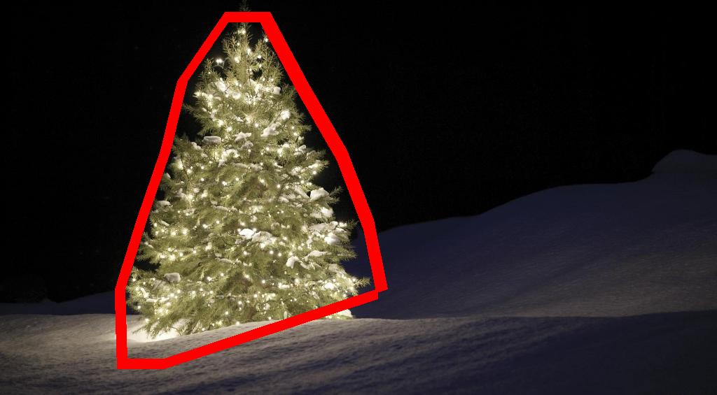
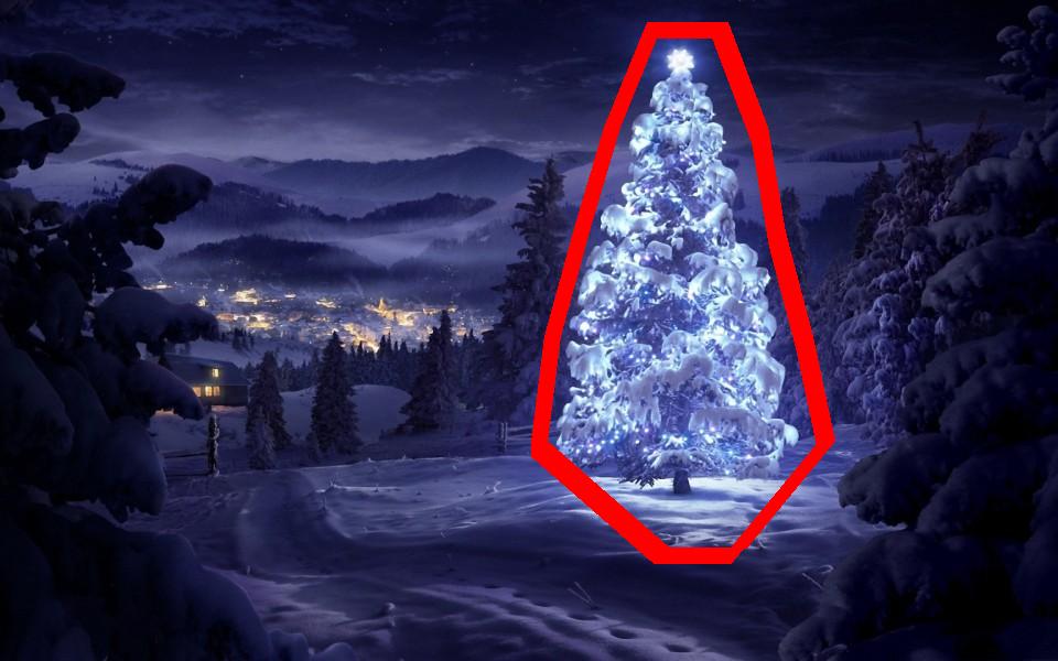
我正在寻找可以用任何编程语言编写的东西， 只要它只使用开源技术。 该解决scheme必须在此问题上共享的映像进行testing。 有6个input图像 ，答案应显示处理每个图像的结果。 最后，对于每个输出图像 ，都必须绘制红线以包围检测到的树。

你将如何去编程检测这些图像中的树？

Answer 1

我有一个我认为有趣的方法，与其他方法有所不同。 与其他一些方法相比，我的方法的主要区别在于如何执行图像分割步骤 – 我使用Python的scikit-learn中的DBSCAN聚类algorithm; 它对于find可能不一定具有单个明确质心的某些非晶形状进行了优化。

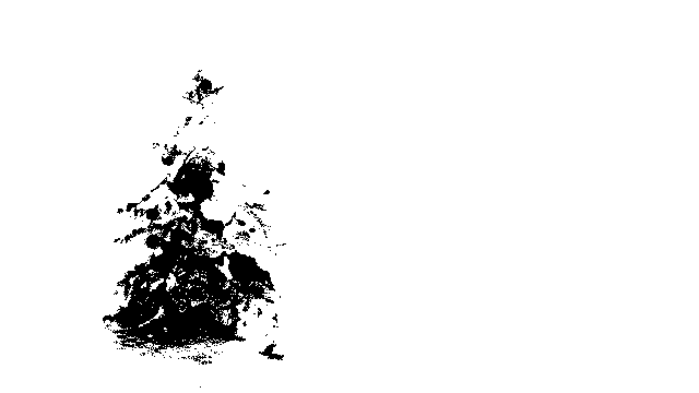
在顶层，我的方法相当简单，可以分解成大约3个步骤。 首先我应用一个门槛（或者实际上是两个独立和不同门槛的逻辑“或”）。 和许多其他答案一样，我假设圣诞树将是场景中更明亮的对象之一，所以第一个阈值只是一个简单的单色亮度testing; 任何在0-255比例（黑色为0，白色为255）上值大于220的像素都将保存为二进制黑白图像。 第二个门槛试图寻找红色和黄色的灯光，这在六个图像的左上angular和右下angular的树木尤其突出，并且与大多数照片中stream行的蓝绿色背景相得益彰。 我将rgb图像转换为hsv空间，并且要求0.0-1.0比例（大致对应于黄色和绿色之间的边界）或大于0.95（对应于紫色和红色之间的边界）的色调小于0.2，另外我需要明亮饱和的颜色：饱和度和数值都必须在0.7以上。 两个阈值过程的结果在逻辑上“或”在一起，并且得到的黑白二进制图像的matrix如下所示：

您可以清楚地看到，每个图像都有一个与每棵树的位置大致相对应的大的像素集合，另外还有一些图像也有一些小的集群，对应于某些build筑物的窗户中的灯光，在地平线上的背景场景。 下一步是让计算机识别这些是独立的群集，并使用群集成员资格ID号正确标记每个像素。

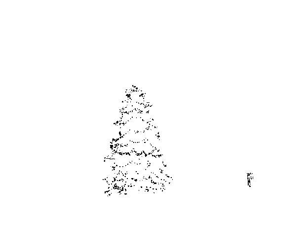
为了这个任务，我select了DBSCAN 。 对于DBSCAN的典型行为，相对于其他集群algorithm， 这里有一个相当不错的视觉比较。 正如我刚才所说，它与无定形的形状相得益彰。 这里显示了DBSCAN的输出，每个群集以不同的颜色绘制：

看这个结果时有几件事要注意。 首先，DBSCAN要求用户设置一个“邻近”参数以调节其行为，这有效地控制了一对点必须分离的程度，以便algorithm声明一个新的分离的聚类，而不是将testing点聚集到一个已经存在的集群。 我把这个值设置为每个图像对angular线大小的0.04倍。 由于图像的大小从大约VGA到大约1080，所以这种尺度相关的定义是至关重要的。

另一点值得注意的是，在scikit-learn中实现的DBSCANalgorithm具有内存限制，对于本示例中的一些较大的图像而言，这是相当具有挑战性的。 因此，对于一些较大的图像，我实际上必须对每个群集进行“抽取”（即只保留每个像素的第3或第4个像素），以便保持在这个极限内。 作为这种剔除过程的结果，其余的单个稀疏像素在一些较大的图像上难以看到。 因此，仅用于显示目的，上述图像中的彩色编码的像素已经被有效地“扩张”了，使得它们更加突出。 为了叙事的缘故，这完全是一种整容手术。 尽pipe在我的代码中有一些评论提到了这个扩展，但是请放心，它与任何实际上很重要的计算都没有关系。

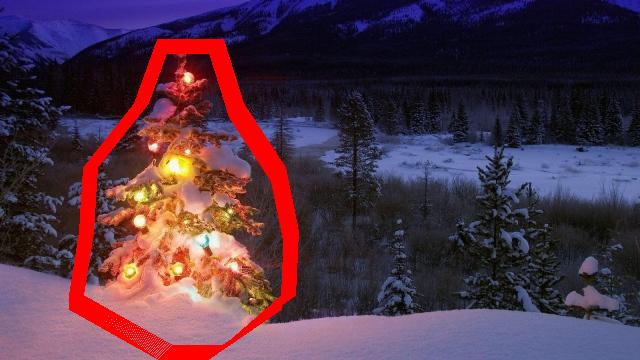
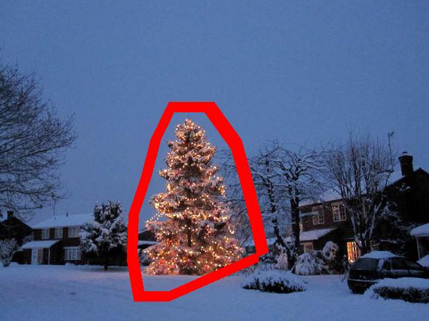
一旦簇被识别和标记，第三步也是最后一步很简单：我只是在每个图像中取最大的簇（在这种情况下，我select以成员像素总数来衡量“大小”，尽pipe可以就像使用某种度量物理范围的度量types一样简单）并计算该群集的凸包。 凸包然后变成树边界。 通过这种方法计算的六个凸包以红色显示如下：

源代码是为Python 2.7.6编写的，它取决于numpy ， scipy ， matplotlib和scikit-learn 。 我把它分成两部分。 第一部分负责实际的image processing：

from PIL import Image import numpy as np import scipy as sp import matplotlib.colors as colors from sklearn.cluster import DBSCAN from math import ceil, sqrt """ Inputs: rgbimg: [M,N,3] numpy array containing (uint, 0-255) color image hueleftthr: Scalar constant to select maximum allowed hue in the yellow-green region huerightthr: Scalar constant to select minimum allowed hue in the blue-purple region satthr: Scalar constant to select minimum allowed saturation valthr: Scalar constant to select minimum allowed value monothr: Scalar constant to select minimum allowed monochrome brightness maxpoints: Scalar constant maximum number of pixels to forward to the DBSCAN clustering algorithm proxthresh: Proximity threshold to use for DBSCAN, as a fraction of the diagonal size of the image Outputs: borderseg: [K,2,2] Nested list containing K pairs of x- and y- pixel values for drawing the tree border X: [P,2] List of pixels that passed the threshold step labels: [Q,2] List of cluster labels for points in Xslice (see below) Xslice: [Q,2] Reduced list of pixels to be passed to DBSCAN """ def findtree(rgbimg, hueleftthr=0.2, huerightthr=0.95, satthr=0.7, valthr=0.7, monothr=220, maxpoints=5000, proxthresh=0.04): # Convert rgb image to monochrome for gryimg = np.asarray(Image.fromarray(rgbimg).convert('L')) # Convert rgb image (uint, 0-255) to hsv (float, 0.0-1.0) hsvimg = colors.rgb_to_hsv(rgbimg.astype(float)/255) # Initialize binary thresholded image binimg = np.zeros((rgbimg.shape[0], rgbimg.shape[1])) # Find pixels with hue<0.2 or hue>0.95 (red or yellow) and saturation/value # both greater than 0.7 (saturated and bright)--tends to coincide with # ornamental lights on trees in some of the images boolidx = np.logical_and( np.logical_and( np.logical_or((hsvimg[:,:,0] < hueleftthr), (hsvimg[:,:,0] > huerightthr)), (hsvimg[:,:,1] > satthr)), (hsvimg[:,:,2] > valthr)) # Find pixels that meet hsv criterion binimg[np.where(boolidx)] = 255 # Add pixels that meet grayscale brightness criterion binimg[np.where(gryimg > monothr)] = 255 # Prepare thresholded points for DBSCAN clustering algorithm X = np.transpose(np.where(binimg == 255)) Xslice = X nsample = len(Xslice) if nsample > maxpoints: # Make sure number of points does not exceed DBSCAN maximum capacity Xslice = X[range(0,nsample,int(ceil(float(nsample)/maxpoints)))] # Translate DBSCAN proximity threshold to units of pixels and run DBSCAN pixproxthr = proxthresh * sqrt(binimg.shape[0]**2 + binimg.shape[1]**2) db = DBSCAN(eps=pixproxthr, min_samples=10).fit(Xslice) labels = db.labels_.astype(int) # Find the largest cluster (ie, with most points) and obtain convex hull unique_labels = set(labels) maxclustpt = 0 for k in unique_labels: class_members = [index[0] for index in np.argwhere(labels == k)] if len(class_members) > maxclustpt: points = Xslice[class_members] hull = sp.spatial.ConvexHull(points) maxclustpt = len(class_members) borderseg = [[points[simplex,0], points[simplex,1]] for simplex in hull.simplices] return borderseg, X, labels, Xslice 

第二部分是一个用户级脚本，它调用第一个文件并生成所有上面的图：

 #!/usr/bin/env python from PIL import Image import numpy as np import matplotlib.pyplot as plt import matplotlib.cm as cm from findtree import findtree # Image files to process fname = ['nmzwj.png', 'aVZhC.png', '2K9EF.png', 'YowlH.png', '2y4o5.png', 'FWhSP.png'] # Initialize figures fgsz = (16,7) figthresh = plt.figure(figsize=fgsz, facecolor='w') figclust = plt.figure(figsize=fgsz, facecolor='w') figcltwo = plt.figure(figsize=fgsz, facecolor='w') figborder = plt.figure(figsize=fgsz, facecolor='w') figthresh.canvas.set_window_title('Thresholded HSV and Monochrome Brightness') figclust.canvas.set_window_title('DBSCAN Clusters (Raw Pixel Output)') figcltwo.canvas.set_window_title('DBSCAN Clusters (Slightly Dilated for Display)') figborder.canvas.set_window_title('Trees with Borders') for ii, name in zip(range(len(fname)), fname): # Open the file and convert to rgb image rgbimg = np.asarray(Image.open(name)) # Get the tree borders as well as a bunch of other intermediate values # that will be used to illustrate how the algorithm works borderseg, X, labels, Xslice = findtree(rgbimg) # Display thresholded images axthresh = figthresh.add_subplot(2,3,ii+1) axthresh.set_xticks([]) axthresh.set_yticks([]) binimg = np.zeros((rgbimg.shape[0], rgbimg.shape[1])) for v, h in X: binimg[v,h] = 255 axthresh.imshow(binimg, interpolation='nearest', cmap='Greys') # Display color-coded clusters axclust = figclust.add_subplot(2,3,ii+1) # Raw version axclust.set_xticks([]) axclust.set_yticks([]) axcltwo = figcltwo.add_subplot(2,3,ii+1) # Dilated slightly for display only axcltwo.set_xticks([]) axcltwo.set_yticks([]) axcltwo.imshow(binimg, interpolation='nearest', cmap='Greys') clustimg = np.ones(rgbimg.shape) unique_labels = set(labels) # Generate a unique color for each cluster plcol = cm.rainbow_r(np.linspace(0, 1, len(unique_labels))) for lbl, pix in zip(labels, Xslice): for col, unqlbl in zip(plcol, unique_labels): if lbl == unqlbl: # Cluster label of -1 indicates no cluster membership; # override default color with black if lbl == -1: col = [0.0, 0.0, 0.0, 1.0] # Raw version for ij in range(3): clustimg[pix[0],pix[1],ij] = col[ij] # Dilated just for display axcltwo.plot(pix[1], pix[0], 'o', markerfacecolor=col, markersize=1, markeredgecolor=col) axclust.imshow(clustimg) axcltwo.set_xlim(0, binimg.shape[1]-1) axcltwo.set_ylim(binimg.shape[0], -1) # Plot original images with read borders around the trees axborder = figborder.add_subplot(2,3,ii+1) axborder.set_axis_off() axborder.imshow(rgbimg, interpolation='nearest') for vseg, hseg in borderseg: axborder.plot(hseg, vseg, 'r-', lw=3) axborder.set_xlim(0, binimg.shape[1]-1) axborder.set_ylim(binimg.shape[0], -1) plt.show() 

Answer 2

编辑注意：我编辑这篇文章（i）按照要求单独处理每个树图像，（ii）考虑对象的亮度和形状，以提高结果的质量。

---

下面介绍一种考虑物体亮度和形状的方法。 换句话说，它寻找具有三angular形形状和明亮度的物体。 它是用Java实现的，使用Marvinimage processing框架。

第一步是颜色阈值。 这里的目标是将分析的重点放在明亮亮度的物体上。

输出图像：

other/trees/tree_1threshold.png other/trees/tree_2threshold.png http://marvinproject.sourceforge.net/other/trees/tree_3threshold。; PNG

其他链接 PNG

源代码：

 public class ChristmasTree { private MarvinImagePlugin fill = MarvinPluginLoader.loadImagePlugin("org.marvinproject.image.fill.boundaryFill"); private MarvinImagePlugin threshold = MarvinPluginLoader.loadImagePlugin("org.marvinproject.image.color.thresholding"); private MarvinImagePlugin invert = MarvinPluginLoader.loadImagePlugin("org.marvinproject.image.color.invert"); private MarvinImagePlugin dilation = MarvinPluginLoader.loadImagePlugin("org.marvinproject.image.morphological.dilation"); public ChristmasTree(){ MarvinImage tree; // Iterate each image for(int i=1; i<=6; i++){ tree = MarvinImageIO.loadImage("./res/trees/tree"+i+".png"); // 1. Threshold threshold.setAttribute("threshold", 200); threshold.process(tree.clone(), tree); } } public static void main(String[] args) { new ChristmasTree(); } } 

在第二步，图像中最亮的点被扩大，以形成形状。 这个过程的结果是具有明显亮度的物体的可能形状。 应用填充分段，检测到断开的形状。

输出图像：

其他链接 PNG

其他链接 PNG

源代码：

 public class ChristmasTree { private MarvinImagePlugin fill = MarvinPluginLoader.loadImagePlugin("org.marvinproject.image.fill.boundaryFill"); private MarvinImagePlugin threshold = MarvinPluginLoader.loadImagePlugin("org.marvinproject.image.color.thresholding"); private MarvinImagePlugin invert = MarvinPluginLoader.loadImagePlugin("org.marvinproject.image.color.invert"); private MarvinImagePlugin dilation = MarvinPluginLoader.loadImagePlugin("org.marvinproject.image.morphological.dilation"); public ChristmasTree(){ MarvinImage tree; // Iterate each image for(int i=1; i<=6; i++){ tree = MarvinImageIO.loadImage("./res/trees/tree"+i+".png"); // 1. Threshold threshold.setAttribute("threshold", 200); threshold.process(tree.clone(), tree); // 2. Dilate invert.process(tree.clone(), tree); tree = MarvinColorModelConverter.rgbToBinary(tree, 127); MarvinImageIO.saveImage(tree, "./res/trees/new/tree_"+i+"threshold.png"); dilation.setAttribute("matrix", MarvinMath.getTrueMatrix(50, 50)); dilation.process(tree.clone(), tree); MarvinImageIO.saveImage(tree, "./res/trees/new/tree_"+1+"_dilation.png"); tree = MarvinColorModelConverter.binaryToRgb(tree); // 3. Segment shapes MarvinImage trees2 = tree.clone(); fill(tree, trees2); MarvinImageIO.saveImage(trees2, "./res/trees/new/tree_"+i+"_fill.png"); } private void fill(MarvinImage imageIn, MarvinImage imageOut){ boolean found; int color= 0xFFFF0000; while(true){ found=false; Outerloop: for(int y=0; y<imageIn.getHeight(); y++){ for(int x=0; x<imageIn.getWidth(); x++){ if(imageOut.getIntComponent0(x, y) == 0){ fill.setAttribute("x", x); fill.setAttribute("y", y); fill.setAttribute("color", color); fill.setAttribute("threshold", 120); fill.process(imageIn, imageOut); color = newColor(color); found = true; break Outerloop; } } } if(!found){ break; } } } private int newColor(int color){ int red = (color & 0x00FF0000) >> 16; int green = (color & 0x0000FF00) >> 8; int blue = (color & 0x000000FF); if(red <= green && red <= blue){ red+=5; } else if(green <= red && green <= blue){ green+=5; } else{ blue+=5; } return 0xFF000000 + (red << 16) + (green << 8) + blue; } public static void main(String[] args) { new ChristmasTree(); } } 

如输出图像所示，检测到多个形状。 在这个问题中，图像中只有几个亮点。 但是，这种方法是为了处理更复杂的情况而实施的。

在下一步中，分析每个形状。 一个简单的algorithm用类似于三angular形的模式检测形状。 该algorithm逐行分析对象形状。 如果每条形状线的质量中心几乎相同（给定一个阈值），质量随着y的增加而增加，则该物体呈三angular形状。 形状线的质量是属于该形状的该行中的像素的数量。 想象一下你水平切割对象并分析每个水平段。 如果它们是相互集中的，并且线性模式中从第一个段到最后一个段的长度增加，则可能有一个类似于三angular形的对象。

源代码：

 private int[] detectTrees(MarvinImage image){ HashSet<Integer> analysed = new HashSet<Integer>(); boolean found; while(true){ found = false; for(int y=0; y<image.getHeight(); y++){ for(int x=0; x<image.getWidth(); x++){ int color = image.getIntColor(x, y); if(!analysed.contains(color)){ if(isTree(image, color)){ return getObjectRect(image, color); } analysed.add(color); found=true; } } } if(!found){ break; } } return null; } private boolean isTree(MarvinImage image, int color){ int mass[][] = new int[image.getHeight()][2]; int yStart=-1; int xStart=-1; for(int y=0; y<image.getHeight(); y++){ int mc = 0; int xs=-1; int xe=-1; for(int x=0; x<image.getWidth(); x++){ if(image.getIntColor(x, y) == color){ mc++; if(yStart == -1){ yStart=y; xStart=x; } if(xs == -1){ xs = x; } if(x > xe){ xe = x; } } } mass[y][0] = xs; mass[y][3] = xe; mass[y][4] = mc; } int validLines=0; for(int y=0; y<image.getHeight(); y++){ if ( mass[y][5] > 0 && Math.abs(((mass[y][0]+mass[y][6])/2)-xStart) <= 50 && mass[y][7] >= (mass[yStart][8] + (y-yStart)*0.3) && mass[y][9] <= (mass[yStart][10] + (y-yStart)*1.5) ) { validLines++; } } if(validLines > 100){ return true; } return false; } 

最后，如下所示，在原始图像中突出显示每个形状与三angular形相似并具有明显亮度的位置，在这种情况下为圣诞树。

最终输出图像：

other/trees/tree_1_out_2.jpg other/trees/tree_2_out_2.jpg http://marvinproject.sourceforge.net/other/trees/tree_3_out_2。; JPG

other/trees/tree_4_out_2.jpg other/trees/tree_5_out_2.jpg http://marvinproject.sourceforge.net/other/trees/tree_6_out_2。; JPG

最终源代码：

 public class ChristmasTree { private MarvinImagePlugin fill = MarvinPluginLoader.loadImagePlugin("org.marvinproject.image.fill.boundaryFill"); private MarvinImagePlugin threshold = MarvinPluginLoader.loadImagePlugin("org.marvinproject.image.color.thresholding"); private MarvinImagePlugin invert = MarvinPluginLoader.loadImagePlugin("org.marvinproject.image.color.invert"); private MarvinImagePlugin dilation = MarvinPluginLoader.loadImagePlugin("org.marvinproject.image.morphological.dilation"); public ChristmasTree(){ MarvinImage tree; // Iterate each image for(int i=1; i<=6; i++){ tree = MarvinImageIO.loadImage("./res/trees/tree"+i+".png"); // 1. Threshold threshold.setAttribute("threshold", 200); threshold.process(tree.clone(), tree); // 2. Dilate invert.process(tree.clone(), tree); tree = MarvinColorModelConverter.rgbToBinary(tree, 127); MarvinImageIO.saveImage(tree, "./res/trees/new/tree_"+i+"threshold.png"); dilation.setAttribute("matrix", MarvinMath.getTrueMatrix(50, 50)); dilation.process(tree.clone(), tree); MarvinImageIO.saveImage(tree, "./res/trees/new/tree_"+1+"_dilation.png"); tree = MarvinColorModelConverter.binaryToRgb(tree); // 3. Segment shapes MarvinImage trees2 = tree.clone(); fill(tree, trees2); MarvinImageIO.saveImage(trees2, "./res/trees/new/tree_"+i+"_fill.png"); // 4. Detect tree-like shapes int[] rect = detectTrees(trees2); // 5. Draw the result MarvinImage original = MarvinImageIO.loadImage("./res/trees/tree"+i+".png"); drawBoundary(trees2, original, rect); MarvinImageIO.saveImage(original, "./res/trees/new/tree_"+i+"_out_2.jpg"); } } private void drawBoundary(MarvinImage shape, MarvinImage original, int[] rect){ int yLines[] = new int[6]; yLines[0] = rect[1]; yLines[1] = rect[1]+(int)((rect[3]/5)); yLines[2] = rect[1]+((rect[3]/5)*2); yLines[3] = rect[1]+((rect[3]/5)*3); yLines[4] = rect[1]+(int)((rect[3]/5)*4); yLines[5] = rect[1]+rect[3]; List<Point> points = new ArrayList<Point>(); for(int i=0; i<yLines.length; i++){ boolean in=false; Point startPoint=null; Point endPoint=null; for(int x=rect[0]; x<rect[0]+rect[2]; x++){ if(shape.getIntColor(x, yLines[i]) != 0xFFFFFFFF){ if(!in){ if(startPoint == null){ startPoint = new Point(x, yLines[i]); } } in = true; } else{ if(in){ endPoint = new Point(x, yLines[i]); } in = false; } } if(endPoint == null){ endPoint = new Point((rect[0]+rect[2])-1, yLines[i]); } points.add(startPoint); points.add(endPoint); } drawLine(points.get(0).x, points.get(0).y, points.get(1).x, points.get(1).y, 15, original); drawLine(points.get(1).x, points.get(1).y, points.get(3).x, points.get(3).y, 15, original); drawLine(points.get(3).x, points.get(3).y, points.get(5).x, points.get(5).y, 15, original); drawLine(points.get(5).x, points.get(5).y, points.get(7).x, points.get(7).y, 15, original); drawLine(points.get(7).x, points.get(7).y, points.get(9).x, points.get(9).y, 15, original); drawLine(points.get(9).x, points.get(9).y, points.get(11).x, points.get(11).y, 15, original); drawLine(points.get(11).x, points.get(11).y, points.get(10).x, points.get(10).y, 15, original); drawLine(points.get(10).x, points.get(10).y, points.get(8).x, points.get(8).y, 15, original); drawLine(points.get(8).x, points.get(8).y, points.get(6).x, points.get(6).y, 15, original); drawLine(points.get(6).x, points.get(6).y, points.get(4).x, points.get(4).y, 15, original); drawLine(points.get(4).x, points.get(4).y, points.get(2).x, points.get(2).y, 15, original); drawLine(points.get(2).x, points.get(2).y, points.get(0).x, points.get(0).y, 15, original); } private void drawLine(int x1, int y1, int x2, int y2, int length, MarvinImage image){ int lx1, lx2, ly1, ly2; for(int i=0; i<length; i++){ lx1 = (x1+i >= image.getWidth() ? (image.getWidth()-1)-i: x1); lx2 = (x2+i >= image.getWidth() ? (image.getWidth()-1)-i: x2); ly1 = (y1+i >= image.getHeight() ? (image.getHeight()-1)-i: y1); ly2 = (y2+i >= image.getHeight() ? (image.getHeight()-1)-i: y2); image.drawLine(lx1+i, ly1, lx2+i, ly2, Color.red); image.drawLine(lx1, ly1+i, lx2, ly2+i, Color.red); } } private void fillRect(MarvinImage image, int[] rect, int length){ for(int i=0; i<length; i++){ image.drawRect(rect[0]+i, rect[1]+i, rect[2]-(i*2), rect[3]-(i*2), Color.red); } } private void fill(MarvinImage imageIn, MarvinImage imageOut){ boolean found; int color= 0xFFFF0000; while(true){ found=false; Outerloop: for(int y=0; y<imageIn.getHeight(); y++){ for(int x=0; x<imageIn.getWidth(); x++){ if(imageOut.getIntComponent0(x, y) == 0){ fill.setAttribute("x", x); fill.setAttribute("y", y); fill.setAttribute("color", color); fill.setAttribute("threshold", 120); fill.process(imageIn, imageOut); color = newColor(color); found = true; break Outerloop; } } } if(!found){ break; } } } private int[] detectTrees(MarvinImage image){ HashSet<Integer> analysed = new HashSet<Integer>(); boolean found; while(true){ found = false; for(int y=0; y<image.getHeight(); y++){ for(int x=0; x<image.getWidth(); x++){ int color = image.getIntColor(x, y); if(!analysed.contains(color)){ if(isTree(image, color)){ return getObjectRect(image, color); } analysed.add(color); found=true; } } } if(!found){ break; } } return null; } private boolean isTree(MarvinImage image, int color){ int mass[][] = new int[image.getHeight()][11]; int yStart=-1; int xStart=-1; for(int y=0; y<image.getHeight(); y++){ int mc = 0; int xs=-1; int xe=-1; for(int x=0; x<image.getWidth(); x++){ if(image.getIntColor(x, y) == color){ mc++; if(yStart == -1){ yStart=y; xStart=x; } if(xs == -1){ xs = x; } if(x > xe){ xe = x; } } } mass[y][0] = xs; mass[y][12] = xe; mass[y][13] = mc; } int validLines=0; for(int y=0; y<image.getHeight(); y++){ if ( mass[y][14] > 0 && Math.abs(((mass[y][0]+mass[y][15])/2)-xStart) <= 50 && mass[y][16] >= (mass[yStart][17] + (y-yStart)*0.3) && mass[y][18] <= (mass[yStart][19] + (y-yStart)*1.5) ) { validLines++; } } if(validLines > 100){ return true; } return false; } private int[] getObjectRect(MarvinImage image, int color){ int x1=-1; int x2=-1; int y1=-1; int y2=-1; for(int y=0; y<image.getHeight(); y++){ for(int x=0; x<image.getWidth(); x++){ if(image.getIntColor(x, y) == color){ if(x1 == -1 || x < x1){ x1 = x; } if(x2 == -1 || x > x2){ x2 = x; } if(y1 == -1 || y < y1){ y1 = y; } if(y2 == -1 || y > y2){ y2 = y; } } } } return new int[]{x1, y1, (x2-x1), (y2-y1)}; } private int newColor(int color){ int red = (color & 0x00FF0000) >> 16; int green = (color & 0x0000FF00) >> 8; int blue = (color & 0x000000FF); if(red <= green && red <= blue){ red+=5; } else if(green <= red && green <= blue){ green+=30; } else{ blue+=30; } return 0xFF000000 + (red << 16) + (green << 8) + blue; } public static void main(String[] args) { new ChristmasTree(); } } 

这种方法的优点是，它可能会处理包含其他发光物体的图像，因为它分析了物体的形状。

圣诞节快乐！

---

编辑注2

关于这个解决scheme的输出图像和其他一些的相似性有一个讨论。 事实上，他们非常相似。 但是这种方法不只是分割对象。 它也从某种意义上分析了物体的形状。 它可以处理同一场景中的多个发光物体。 事实上，圣诞树不需要是最亮的。 我只是为了丰富讨论。 样品中存在一个偏差，只是寻找最明亮的物体，你会发现树木。 但是，我们现在真的要停止讨论吗？ 在这一点上，电脑能够在多大程度上识别类似圣诞树的物体呢？ 我们试着缩小这个差距。

下面给出一个结果来澄清这一点：

input图像

产量

Answer 3

这是我简单和愚蠢的解决scheme。 它是基于这样一个假设，那就是树将是图中最明亮和最大的东西。

 //g++ -Wall -pedantic -ansi -O2 -pipe -s -o christmas_tree christmas_tree.cpp `pkg-config --cflags --libs opencv` #include <opencv2/imgproc/imgproc.hpp> #include <opencv2/highgui/highgui.hpp> #include <iostream> using namespace cv; using namespace std; int main(int argc,char *argv[]) { Mat original,tmp,tmp1; vector <vector<Point> > contours; Moments m; Rect boundrect; Point2f center; double radius, max_area=0,tmp_area=0; unsigned int j, k; int i; for(i = 1; i < argc; ++i) { original = imread(argv[i]); if(original.empty()) { cerr << "Error"<<endl; return -1; } GaussianBlur(original, tmp, Size(3, 3), 0, 0, BORDER_DEFAULT); erode(tmp, tmp, Mat(), Point(-1, -1), 10); cvtColor(tmp, tmp, CV_BGR2HSV); inRange(tmp, Scalar(0, 0, 0), Scalar(180, 255, 200), tmp); dilate(original, tmp1, Mat(), Point(-1, -1), 15); cvtColor(tmp1, tmp1, CV_BGR2HLS); inRange(tmp1, Scalar(0, 185, 0), Scalar(180, 255, 255), tmp1); dilate(tmp1, tmp1, Mat(), Point(-1, -1), 10); bitwise_and(tmp, tmp1, tmp1); findContours(tmp1, contours, CV_RETR_EXTERNAL, CV_CHAIN_APPROX_SIMPLE); max_area = 0; j = 0; for(k = 0; k < contours.size(); k++) { tmp_area = contourArea(contours[k]); if(tmp_area > max_area) { max_area = tmp_area; j = k; } } tmp1 = Mat::zeros(original.size(),CV_8U); approxPolyDP(contours[j], contours[j], 30, true); drawContours(tmp1, contours, j, Scalar(255,255,255), CV_FILLED); m = moments(contours[j]); boundrect = boundingRect(contours[j]); center = Point2f(m.m10/m.m00, m.m01/m.m00); radius = (center.y - (boundrect.tl().y))/4.0*3.0; Rect heightrect(center.x-original.cols/5, boundrect.tl().y, original.cols/5*2, boundrect.size().height); tmp = Mat::zeros(original.size(), CV_8U); rectangle(tmp, heightrect, Scalar(255, 255, 255), -1); circle(tmp, center, radius, Scalar(255, 255, 255), -1); bitwise_and(tmp, tmp1, tmp1); findContours(tmp1, contours, CV_RETR_EXTERNAL, CV_CHAIN_APPROX_SIMPLE); max_area = 0; j = 0; for(k = 0; k < contours.size(); k++) { tmp_area = contourArea(contours[k]); if(tmp_area > max_area) { max_area = tmp_area; j = k; } } approxPolyDP(contours[j], contours[j], 30, true); convexHull(contours[j], contours[j]); drawContours(original, contours, j, Scalar(0, 0, 255), 3); namedWindow(argv[i], CV_WINDOW_NORMAL|CV_WINDOW_KEEPRATIO|CV_GUI_EXPANDED); imshow(argv[i], original); waitKey(0); destroyWindow(argv[i]); } return 0; } 

第一步是检测图片中最亮的像素，但是我们必须区分树本身和reflection光的雪。 在这里，我们尝试排除在颜色代码上使用真正简单的filter的雪花：

 GaussianBlur(original, tmp, Size(3, 3), 0, 0, BORDER_DEFAULT); erode(tmp, tmp, Mat(), Point(-1, -1), 10); cvtColor(tmp, tmp, CV_BGR2HSV); inRange(tmp, Scalar(0, 0, 0), Scalar(180, 255, 200), tmp); 

然后我们find每个“明亮”像素：

 dilate(original, tmp1, Mat(), Point(-1, -1), 15); cvtColor(tmp1, tmp1, CV_BGR2HLS); inRange(tmp1, Scalar(0, 185, 0), Scalar(180, 255, 255), tmp1); dilate(tmp1, tmp1, Mat(), Point(-1, -1), 10); 

最后我们join两个结果：

 bitwise_and(tmp, tmp1, tmp1); 

现在我们寻找最大的亮点：

 findContours(tmp1, contours, CV_RETR_EXTERNAL, CV_CHAIN_APPROX_SIMPLE); max_area = 0; j = 0; for(k = 0; k < contours.size(); k++) { tmp_area = contourArea(contours[k]); if(tmp_area > max_area) { max_area = tmp_area; j = k; } } tmp1 = Mat::zeros(original.size(),CV_8U); approxPolyDP(contours[j], contours[j], 30, true); drawContours(tmp1, contours, j, Scalar(255,255,255), CV_FILLED); 

现在我们已经差不多完成了，但是由于积雪，还是有一些不完美之处。 为了将它们切掉，我们将使用圆形和矩形来构build一个蒙版来近似树的形状以删除不需要的部分：

 m = moments(contours[j]); boundrect = boundingRect(contours[j]); center = Point2f(m.m10/m.m00, m.m01/m.m00); radius = (center.y - (boundrect.tl().y))/4.0*3.0; Rect heightrect(center.x-original.cols/5, boundrect.tl().y, original.cols/5*2, boundrect.size().height); tmp = Mat::zeros(original.size(), CV_8U); rectangle(tmp, heightrect, Scalar(255, 255, 255), -1); circle(tmp, center, radius, Scalar(255, 255, 255), -1); bitwise_and(tmp, tmp1, tmp1); 

最后一步是find我们的树的轮廓，并将其绘制在原始图片上。

 findContours(tmp1, contours, CV_RETR_EXTERNAL, CV_CHAIN_APPROX_SIMPLE); max_area = 0; j = 0; for(k = 0; k < contours.size(); k++) { tmp_area = contourArea(contours[k]); if(tmp_area > max_area) { max_area = tmp_area; j = k; } } approxPolyDP(contours[j], contours[j], 30, true); convexHull(contours[j], contours[j]); drawContours(original, contours, j, Scalar(0, 0, 255), 3); 

我很抱歉，但目前我有一个不好的连接，所以我不能上传图片。 我会尽力做到这一点。

圣诞节快乐。

编辑：

这里有一些最终输出的图片：

Answer 4

我在Matlab R2007a中编写了代码。 我用k-means粗略地提取了圣诞树。 我只会用一个图像来展示我的中间结果，最后的结果将会是六个。

首先，我将RGB空间映射到Lab空间，这可以增强b通道中红色的对比度：

 colorTransform = makecform('srgb2lab'); I = applycform(I, colorTransform); L = double(I(:,:,1)); a = double(I(:,:,2)); b = double(I(:,:,3)); 

除了色彩空间的特征之外，我还使用了与邻域相关的纹理特征，而不是每个像素本身。 在这里，我将来自3个原始通道（R，G，B）的强度线性组合。 我之所以这样格式化，是因为图片中的圣诞树上都有红灯，有时也有绿/有时是蓝的照明。

 R=double(Irgb(:,:,1)); G=double(Irgb(:,:,2)); B=double(Irgb(:,:,3)); I0 = (3*R + max(G,B)-min(G,B))/2; 

我在I0上应用了一个3X3的局部二值模式，用中心像素作为阈值，通过计算阈值以上的平均像素强度值与其下面的平均值之间的差值来获得对比度。

 I0_copy = zeros(size(I0)); for i = 2 : size(I0,1) - 1 for j = 2 : size(I0,2) - 1 tmp = I0(i-1:i+1,j-1:j+1) >= I0(i,j); I0_copy(i,j) = mean(mean(tmp.*I0(i-1:i+1,j-1:j+1))) - ... mean(mean(~tmp.*I0(i-1:i+1,j-1:j+1))); % Contrast end end 

由于我总共有4个特征，所以在我的聚类方法中我selectK = 5。 k-means的代码如下所示（这是来自Andrew Ng博士的机器学习课程，之前我学习过这个课程，我自己也编写了代码）。

 [centroids, idx] = runkMeans(X, initial_centroids, max_iters); mask=reshape(idx,img_size(1),img_size(2)); %%%%%%%%%%%%%%%%%%%%%%%%%%%%%%%%%%%%%%%%%%%%%%%%%%%% function [centroids, idx] = runkMeans(X, initial_centroids, ... max_iters, plot_progress) [mn] = size(X); K = size(initial_centroids, 1); centroids = initial_centroids; previous_centroids = centroids; idx = zeros(m, 1); for i=1:max_iters % For each example in X, assign it to the closest centroid idx = findClosestCentroids(X, centroids); % Given the memberships, compute new centroids centroids = computeCentroids(X, idx, K); end %%%%%%%%%%%%%%%%%%%%%%%%%%%%%%%%%%%%%%%%%%%%%%%%%%%%%%% function idx = findClosestCentroids(X, centroids) K = size(centroids, 1); idx = zeros(size(X,1), 1); for xi = 1:size(X,1) x = X(xi, :); % Find closest centroid for x. best = Inf; for mui = 1:K mu = centroids(mui, :); d = dot(x - mu, x - mu); if d < best best = d; idx(xi) = mui; end end end %%%%%%%%%%%%%%%%%%%%%%%%%%%%%%%%%%% function centroids = computeCentroids(X, idx, K) [mn] = size(X); centroids = zeros(K, n); for mui = 1:K centroids(mui, :) = sum(X(idx == mui, :)) / sum(idx == mui); end 

由于程序在我的电脑上运行得非常慢，我只运行了3次迭代。 通常停止标准是（i）迭代时间至less为10，或者（ii）质心不再变化。 在我的testing中，增加迭代可以更准确地区分背景（天空和树木，天空和build筑物…），但没有显示圣诞树提取中的剧烈变化。 还要注意k-means对随机质心初始化不是免疫的，所以推荐多次运行程序进行比较。

在k-均值之后，select具有最大强度I0的标记区域。 边界追踪被用来提取边界。 对我来说，最后一棵圣诞树是最难提取的，因为这幅图的对比度不如前五。 在我的方法中的另一个问题是，我用Matlab中的边界函数来追踪边界，但有时也包括内部边界，你可以在第3，第5，第6结果中观察到。 圣诞树内的黑暗面不仅没有与照亮的一面聚集在一起，而且还导致了许多微小的内部边界的追踪（ imfill并没有太多改善）。 In all my algorithm still has a lot improvement space.

Some publication s indicates that mean-shift may be more robust than k-means, and many graph-cut based algorithms are also very competitive on complicated boundaries segmentation. I wrote a mean-shift algorithm myself, it seems to better extract the regions without enough light. But mean-shift is a little bit over-segmented, and some strategy of merging is needed. It ran even much slower than k-means in my computer, I am afraid I have to give it up. I eagerly look forward to see others would submit excellent results here with those modern algorithms mentioned above.

Yet I always believe the feature selection is the key component in image segmentation. With a proper feature selection that can maximize the margin between object and background, many segmentation algorithms will definitely work. Different algorithms may improve the result from 1 to 10, but the feature selection may improve it from 0 to 1.

Merry Christmas !

Answer 5

This is my final post using the traditional image processing approaches…

Here I somehow combine my two other proposals, achieving even better results . As a matter of fact I cannot see how these results could be better (especially when you look at the masked images that the method produces).

At the heart of the approach is the combination of three key assumptions :

1. Images should have high fluctuations in the tree regions
2. Images should have higher intensity in the tree regions
3. Background regions should have low intensity and be mostly blue-ish

With these assumptions in mind the method works as follows:

1. Convert the images to HSV
2. Filter the V channel with a LoG filter
3. Apply hard thresholding on LoG filtered image to get 'activity' mask A
4. Apply hard thresholding to V channel to get intensity mask B
5. Apply H channel thresholding to capture low intensity blue-ish regions into background mask C
6. Combine masks using AND to get the final mask
7. Dilate the mask to enlarge regions and connect dispersed pixels
8. Eliminate small regions and get the final mask which will eventually represent only the tree

Here is the code in MATLAB (again, the script loads all jpg images in the current folder and, again, this is far from being an optimized piece of code):

 % clear everything clear; pack; close all; close all hidden; drawnow; clc; % initialization ims=dir('./*.jpg'); imgs={}; images={}; blur_images={}; log_image={}; dilated_image={}; int_image={}; back_image={}; bin_image={}; measurements={}; box={}; num=length(ims); thres_div = 3; for i=1:num, % load original image imgs{end+1}=imread(ims(i).name); % convert to HSV colorspace images{end+1}=rgb2hsv(imgs{i}); % apply laplacian filtering and heuristic hard thresholding val_thres = (max(max(images{i}(:,:,3)))/thres_div); log_image{end+1} = imfilter( images{i}(:,:,3),fspecial('log')) > val_thres; % get the most bright regions of the image int_thres = 0.26*max(max( images{i}(:,:,3))); int_image{end+1} = images{i}(:,:,3) > int_thres; % get the most probable background regions of the image back_image{end+1} = images{i}(:,:,1)>(150/360) & images{i}(:,:,1)<(320/360) & images{i}(:,:,3)<0.5; % compute the final binary image by combining % high 'activity' with high intensity bin_image{end+1} = logical( log_image{i}) & logical( int_image{i}) & ~logical( back_image{i}); % apply morphological dilation to connect distonnected components strel_size = round(0.01*max(size(imgs{i}))); % structuring element for morphological dilation dilated_image{end+1} = imdilate( bin_image{i}, strel('disk',strel_size)); % do some measurements to eliminate small objects measurements{i} = regionprops( logical( dilated_image{i}),'Area','BoundingBox'); % iterative enlargement of the structuring element for better connectivity while length(measurements{i})>14 && strel_size<(min(size(imgs{i}(:,:,1)))/2), strel_size = round( 1.5 * strel_size); dilated_image{i} = imdilate( bin_image{i}, strel('disk',strel_size)); measurements{i} = regionprops( logical( dilated_image{i}),'Area','BoundingBox'); end for m=1:length(measurements{i}) if measurements{i}(m).Area < 0.05*numel( dilated_image{i}) dilated_image{i}( round(measurements{i}(m).BoundingBox(2):measurements{i}(m).BoundingBox(4)+measurements{i}(m).BoundingBox(2)),... round(measurements{i}(m).BoundingBox(1):measurements{i}(m).BoundingBox(3)+measurements{i}(m).BoundingBox(1))) = 0; end end % make sure the dilated image is the same size with the original dilated_image{i} = dilated_image{i}(1:size(imgs{i},1),1:size(imgs{i},2)); % compute the bounding box [y,x] = find( dilated_image{i}); if isempty( y) box{end+1}=[]; else box{end+1} = [ min(x) min(y) max(x)-min(x)+1 max(y)-min(y)+1]; end end %%% additional code to display things for i=1:num, figure; subplot(121); colormap gray; imshow( imgs{i}); if ~isempty(box{i}) hold on; rr = rectangle( 'position', box{i}); set( rr, 'EdgeColor', 'r'); hold off; end subplot(122); imshow( imgs{i}.*uint8(repmat(dilated_image{i},[1 1 3]))); end 

结果

High resolution results still available here!
Even more experiments with additional images can be found here.

Answer 6

…another old fashioned solution – purely based on HSV processing :

1. Convert images to the HSV colorspace
2. Create masks according to heuristics in the HSV (see below)
3. Apply morphological dilation to the mask to connect disconnected areas
4. Discard small areas and horizontal blocks (remember trees are vertical blocks)
5. Compute the bounding box

A word on the heuristics in the HSV processing:

1. everything with Hues (H) between 210 – 320 degrees is discarded as blue-magenta that is supposed to be in the background or in non-relevant areas
2. everything with Values (V) lower that 40% is also discarded as being too dark to be relevant

Of course one may experiment with numerous other possibilities to fine-tune this approach…

Here is the MATLAB code to do the trick (warning: the code is far from being optimized!!! I used techniques not recommended for MATLAB programming just to be able to track anything in the process-this can be greatly optimized):

 % clear everything clear; pack; close all; close all hidden; drawnow; clc; % initialization ims=dir('./*.jpg'); num=length(ims); imgs={}; hsvs={}; masks={}; dilated_images={}; measurements={}; boxs={}; for i=1:num, % load original image imgs{end+1} = imread(ims(i).name); flt_x_size = round(size(imgs{i},2)*0.005); flt_y_size = round(size(imgs{i},1)*0.005); flt = fspecial( 'average', max( flt_y_size, flt_x_size)); imgs{i} = imfilter( imgs{i}, flt, 'same'); % convert to HSV colorspace hsvs{end+1} = rgb2hsv(imgs{i}); % apply a hard thresholding and binary operation to construct the mask masks{end+1} = medfilt2( ~(hsvs{i}(:,:,1)>(210/360) & hsvs{i}(:,:,1)<(320/360))&hsvs{i}(:,:,3)>0.4); % apply morphological dilation to connect distonnected components strel_size = round(0.03*max(size(imgs{i}))); % structuring element for morphological dilation dilated_images{end+1} = imdilate( masks{i}, strel('disk',strel_size)); % do some measurements to eliminate small objects measurements{i} = regionprops( dilated_images{i},'Perimeter','Area','BoundingBox'); for m=1:length(measurements{i}) if (measurements{i}(m).Area < 0.02*numel( dilated_images{i})) || (measurements{i}(m).BoundingBox(3)>1.2*measurements{i}(m).BoundingBox(4)) dilated_images{i}( round(measurements{i}(m).BoundingBox(2):measurements{i}(m).BoundingBox(4)+measurements{i}(m).BoundingBox(2)),... round(measurements{i}(m).BoundingBox(1):measurements{i}(m).BoundingBox(3)+measurements{i}(m).BoundingBox(1))) = 0; end end dilated_images{i} = dilated_images{i}(1:size(imgs{i},1),1:size(imgs{i},2)); % compute the bounding box [y,x] = find( dilated_images{i}); if isempty( y) boxs{end+1}=[]; else boxs{end+1} = [ min(x) min(y) max(x)-min(x)+1 max(y)-min(y)+1]; end end %%% additional code to display things for i=1:num, figure; subplot(121); colormap gray; imshow( imgs{i}); if ~isempty(boxs{i}) hold on; rr = rectangle( 'position', boxs{i}); set( rr, 'EdgeColor', 'r'); hold off; end subplot(122); imshow( imgs{i}.*uint8(repmat(dilated_images{i},[1 1 3]))); end 

结果：

In the results I show the masked image and the bounding box.

Answer 7

My solution steps:

1. Get R channel (from RGB) – all operations we make on this channel:

2. Create Region of Interest (ROI)

   • Threshold R channel with min value 149 (top right image)

   • Dilate result region (middle left image)

3. Detect eges in computed roi. Tree has a lot of edges (middle right image)

   • Dilate result

   • Erode with bigger radius ( bottom left image)

4. Select the biggest (by area) object – it's the result region

5. ConvexHull ( tree is convex polygon ) ( bottom right image )

6. Bounding box (bottom right image – grren box )

Step by step:

The first result – most simple but not in open source software – "Adaptive Vision Studio + Adaptive Vision Library": This is not open source but really fast to prototype:

Whole algorithm to detect christmas tree (11 blocks):

Next step. We want open source solution. Change AVL filters to OpenCV filters: Here I did little changes eg Edge Detection use cvCanny filter, to respect roi i did multiply region image with edges image, to select the biggest element i used findContours + contourArea but idea is the same.

https://www.youtube.com/watch?v=sfjB3MigLH0&index=1&list=UUpSRrkMHNHiLDXgylwhWNQQ

I can't show images with intermediate steps now because I can put only 2 links.

Ok now we use openSource filters but it's not still whole open source. Last step – port to c++ code. I used OpenCV in version 2.4.4

The result of final c++ code is:

c++ code is also quite short:

 #include "opencv2/highgui/highgui.hpp" #include "opencv2/opencv.hpp" #include <algorithm> using namespace cv; int main() { string images[6] = {"..\\1.png","..\\2.png","..\\3.png","..\\4.png","..\\5.png","..\\6.png"}; for(int i = 0; i < 6; ++i) { Mat img, thresholded, tdilated, tmp, tmp1; vector<Mat> channels(3); img = imread(images[i]); split(img, channels); threshold( channels[2], thresholded, 149, 255, THRESH_BINARY); //prepare ROI - threshold dilate( thresholded, tdilated, getStructuringElement( MORPH_RECT, Size(22,22) ) ); //prepare ROI - dilate Canny( channels[2], tmp, 75, 125, 3, true ); //Canny edge detection multiply( tmp, tdilated, tmp1 ); // set ROI dilate( tmp1, tmp, getStructuringElement( MORPH_RECT, Size(20,16) ) ); // dilate erode( tmp, tmp1, getStructuringElement( MORPH_RECT, Size(36,36) ) ); // erode vector<vector<Point> > contours, contours1(1); vector<Point> convex; vector<Vec4i> hierarchy; findContours( tmp1, contours, hierarchy, CV_RETR_TREE, CV_CHAIN_APPROX_SIMPLE, Point(0, 0) ); //get element of maximum area //int bestID = std::max_element( contours.begin(), contours.end(), // []( const vector<Point>& A, const vector<Point>& B ) { return contourArea(A) < contourArea(B); } ) - contours.begin(); int bestID = 0; int bestArea = contourArea( contours[0] ); for( int i = 1; i < contours.size(); ++i ) { int area = contourArea( contours[i] ); if( area > bestArea ) { bestArea = area; bestID = i; } } convexHull( contours[bestID], contours1[0] ); drawContours( img, contours1, 0, Scalar( 100, 100, 255 ), img.rows / 100, 8, hierarchy, 0, Point() ); imshow("image", img ); waitKey(0); } return 0; } 

Answer 8

Some old-fashioned image processing approach…
The idea is based on the assumption that images depict lighted trees on typically darker and smoother backgrounds (or foregrounds in some cases). The lighted tree area is more "energetic" and has higher intensity .
The process is as follows:

1. Convert to graylevel
2. Apply LoG filtering to get the most "active" areas
3. Apply an intentisy thresholding to get the most bright areas
4. Combine the previous 2 to get a preliminary mask
5. Apply a morphological dilation to enlarge areas and connect neighboring components
6. Eliminate small candidate areas according to their area size

What you get is a binary mask and a bounding box for each image.

Here are the results using this naive technique:

Code on MATLAB follows: The code runs on a folder with JPG images. Loads all images and returns detected results.

 % clear everything clear; pack; close all; close all hidden; drawnow; clc; % initialization ims=dir('./*.jpg'); imgs={}; images={}; blur_images={}; log_image={}; dilated_image={}; int_image={}; bin_image={}; measurements={}; box={}; num=length(ims); thres_div = 3; for i=1:num, % load original image imgs{end+1}=imread(ims(i).name); % convert to grayscale images{end+1}=rgb2gray(imgs{i}); % apply laplacian filtering and heuristic hard thresholding val_thres = (max(max(images{i}))/thres_div); log_image{end+1} = imfilter( images{i},fspecial('log')) > val_thres; % get the most bright regions of the image int_thres = 0.26*max(max( images{i})); int_image{end+1} = images{i} > int_thres; % compute the final binary image by combining % high 'activity' with high intensity bin_image{end+1} = log_image{i} .* int_image{i}; % apply morphological dilation to connect distonnected components strel_size = round(0.01*max(size(imgs{i}))); % structuring element for morphological dilation dilated_image{end+1} = imdilate( bin_image{i}, strel('disk',strel_size)); % do some measurements to eliminate small objects measurements{i} = regionprops( logical( dilated_image{i}),'Area','BoundingBox'); for m=1:length(measurements{i}) if measurements{i}(m).Area < 0.05*numel( dilated_image{i}) dilated_image{i}( round(measurements{i}(m).BoundingBox(2):measurements{i}(m).BoundingBox(4)+measurements{i}(m).BoundingBox(2)),... round(measurements{i}(m).BoundingBox(1):measurements{i}(m).BoundingBox(3)+measurements{i}(m).BoundingBox(1))) = 0; end end % make sure the dilated image is the same size with the original dilated_image{i} = dilated_image{i}(1:size(imgs{i},1),1:size(imgs{i},2)); % compute the bounding box [y,x] = find( dilated_image{i}); if isempty( y) box{end+1}=[]; else box{end+1} = [ min(x) min(y) max(x)-min(x)+1 max(y)-min(y)+1]; end end %%% additional code to display things for i=1:num, figure; subplot(121); colormap gray; imshow( imgs{i}); if ~isempty(box{i}) hold on; rr = rectangle( 'position', box{i}); set( rr, 'EdgeColor', 'r'); hold off; end subplot(122); imshow( imgs{i}.*uint8(repmat(dilated_image{i},[1 1 3]))); end 

Answer 9

Using a quite different approach from what I've seen, I created a php script that detects christmas trees by their lights. The result ist always a symmetrical triangle, and if necessary numeric values like the angle ("fatness") of the tree.

The biggest threat to this algorithm obviously are lights next to (in great numbers) or in front of the tree (the greater problem until further optimization). Edit (added): What it can't do: Find out if there's a christmas tree or not, find multiple christmas trees in one image, correctly detect a cristmas tree in the middle of Las Vegas, detect christmas trees that are heavily bent, upside-down or chopped down… 😉

The different stages are:

• Calculate the added brightness (R+G+B) for each pixel
• Add up this value of all 8 neighbouring pixels on top of each pixel
• Rank all pixels by this value (brightest first) – I know, not really subtle…
• Choose N of these, starting from the top, skipping ones that are too close
• Calculate the median of these top N (gives us the approximate center of the tree)
• Start from the median position upwards in a widening search beam for the topmost light from the selected brightest ones (people tend to put at least one light at the very top)
• From there, imagine lines going 60 degrees left and right downwards (christmas trees shouldn't be that fat)
• Decrease those 60 degrees until 20% of the brightest lights are outside this triangle
• Find the light at the very bottom of the triangle, giving you the lower horizontal border of the tree
• 完成

Explanation of the markings:

• Big red cross in the center of the tree: Median of the top N brightest lights
• Dotted line from there upwards: "search beam" for the top of the tree
• Smaller red cross: top of the tree
• Really small red crosses: All of the top N brightest lights
• Red triangle: D'uh!

Source code:

 <?php ini_set('memory_limit', '1024M'); header("Content-type: image/png"); $chosenImage = 6; switch($chosenImage){ case 1: $inputImage = imagecreatefromjpeg("nmzwj.jpg"); break; case 2: $inputImage = imagecreatefromjpeg("2y4o5.jpg"); break; case 3: $inputImage = imagecreatefromjpeg("YowlH.jpg"); break; case 4: $inputImage = imagecreatefromjpeg("2K9Ef.jpg"); break; case 5: $inputImage = imagecreatefromjpeg("aVZhC.jpg"); break; case 6: $inputImage = imagecreatefromjpeg("FWhSP.jpg"); break; case 7: $inputImage = imagecreatefromjpeg("roemerberg.jpg"); break; default: exit(); } // Process the loaded image $topNspots = processImage($inputImage); imagejpeg($inputImage); imagedestroy($inputImage); // Here be functions function processImage($image) { $orange = imagecolorallocate($image, 220, 210, 60); $black = imagecolorallocate($image, 0, 0, 0); $red = imagecolorallocate($image, 255, 0, 0); $maxX = imagesx($image)-1; $maxY = imagesy($image)-1; // Parameters $spread = 1; // Number of pixels to each direction that will be added up $topPositions = 80; // Number of (brightest) lights taken into account $minLightDistance = round(min(array($maxX, $maxY)) / 30); // Minimum number of pixels between the brigtests lights $searchYperX = 5; // spread of the "search beam" from the median point to the top $renderStage = 3; // 1 to 3; exits the process early // STAGE 1 // Calculate the brightness of each pixel (R+G+B) $maxBrightness = 0; $stage1array = array(); for($row = 0; $row <= $maxY; $row++) { $stage1array[$row] = array(); for($col = 0; $col <= $maxX; $col++) { $rgb = imagecolorat($image, $col, $row); $brightness = getBrightnessFromRgb($rgb); $stage1array[$row][$col] = $brightness; if($renderStage == 1){ $brightnessToGrey = round($brightness / 765 * 256); $greyRgb = imagecolorallocate($image, $brightnessToGrey, $brightnessToGrey, $brightnessToGrey); imagesetpixel($image, $col, $row, $greyRgb); } if($brightness > $maxBrightness) { $maxBrightness = $brightness; if($renderStage == 1){ imagesetpixel($image, $col, $row, $red); } } } } if($renderStage == 1) { return; } // STAGE 2 // Add up brightness of neighbouring pixels $stage2array = array(); $maxStage2 = 0; for($row = 0; $row <= $maxY; $row++) { $stage2array[$row] = array(); for($col = 0; $col <= $maxX; $col++) { if(!isset($stage2array[$row][$col])) $stage2array[$row][$col] = 0; // Look around the current pixel, add brightness for($y = $row-$spread; $y <= $row+$spread; $y++) { for($x = $col-$spread; $x <= $col+$spread; $x++) { // Don't read values from outside the image if($x >= 0 && $x <= $maxX && $y >= 0 && $y <= $maxY){ $stage2array[$row][$col] += $stage1array[$y][$x]+10; } } } $stage2value = $stage2array[$row][$col]; if($stage2value > $maxStage2) { $maxStage2 = $stage2value; } } } if($renderStage >= 2){ // Paint the accumulated light, dimmed by the maximum value from stage 2 for($row = 0; $row <= $maxY; $row++) { for($col = 0; $col <= $maxX; $col++) { $brightness = round($stage2array[$row][$col] / $maxStage2 * 255); $greyRgb = imagecolorallocate($image, $brightness, $brightness, $brightness); imagesetpixel($image, $col, $row, $greyRgb); } } } if($renderStage == 2) { return; } // STAGE 3 // Create a ranking of bright spots (like "Top 20") $topN = array(); for($row = 0; $row <= $maxY; $row++) { for($col = 0; $col <= $maxX; $col++) { $stage2Brightness = $stage2array[$row][$col]; $topN[$col.":".$row] = $stage2Brightness; } } arsort($topN); $topNused = array(); $topPositionCountdown = $topPositions; if($renderStage == 3){ foreach ($topN as $key => $val) { if($topPositionCountdown <= 0){ break; } $position = explode(":", $key); foreach($topNused as $usedPosition => $usedValue) { $usedPosition = explode(":", $usedPosition); $distance = abs($usedPosition[0] - $position[0]) + abs($usedPosition[1] - $position[1]); if($distance < $minLightDistance) { continue 2; } } $topNused[$key] = $val; paintCrosshair($image, $position[0], $position[1], $red, 2); $topPositionCountdown--; } } // STAGE 4 // Median of all Top N lights $topNxValues = array(); $topNyValues = array(); foreach ($topNused as $key => $val) { $position = explode(":", $key); array_push($topNxValues, $position[0]); array_push($topNyValues, $position[1]); } $medianXvalue = round(calculate_median($topNxValues)); $medianYvalue = round(calculate_median($topNyValues)); paintCrosshair($image, $medianXvalue, $medianYvalue, $red, 15); // STAGE 5 // Find treetop $filename = 'debug.log'; $handle = fopen($filename, "w"); fwrite($handle, "\n\n STAGE 5"); $treetopX = $medianXvalue; $treetopY = $medianYvalue; $searchXmin = $medianXvalue; $searchXmax = $medianXvalue; $width = 0; for($y = $medianYvalue; $y >= 0; $y--) { fwrite($handle, "\nAt y = ".$y); if(($y % $searchYperX) == 0) { // Modulo $width++; $searchXmin = $medianXvalue - $width; $searchXmax = $medianXvalue + $width; imagesetpixel($image, $searchXmin, $y, $red); imagesetpixel($image, $searchXmax, $y, $red); } foreach ($topNused as $key => $val) { $position = explode(":", $key); // "x:y" if($position[1] != $y){ continue; } if($position[0] >= $searchXmin && $position[0] <= $searchXmax){ $treetopX = $position[0]; $treetopY = $y; } } } paintCrosshair($image, $treetopX, $treetopY, $red, 5); // STAGE 6 // Find tree sides fwrite($handle, "\n\n STAGE 6"); $treesideAngle = 60; // The extremely "fat" end of a christmas tree $treeBottomY = $treetopY; $topPositionsExcluded = 0; $xymultiplier = 0; while(($topPositionsExcluded < ($topPositions / 5)) && $treesideAngle >= 1){ fwrite($handle, "\n\nWe're at angle ".$treesideAngle); $xymultiplier = sin(deg2rad($treesideAngle)); fwrite($handle, "\nMultiplier: ".$xymultiplier); $topPositionsExcluded = 0; foreach ($topNused as $key => $val) { $position = explode(":", $key); fwrite($handle, "\nAt position ".$key); if($position[1] > $treeBottomY) { $treeBottomY = $position[1]; } // Lights above the tree are outside of it, but don't matter if($position[1] < $treetopY){ $topPositionsExcluded++; fwrite($handle, "\nTOO HIGH"); continue; } // Top light will generate division by zero if($treetopY-$position[1] == 0) { fwrite($handle, "\nDIVISION BY ZERO"); continue; } // Lights left end right of it are also not inside fwrite($handle, "\nLight position factor: ".(abs($treetopX-$position[0]) / abs($treetopY-$position[1]))); if((abs($treetopX-$position[0]) / abs($treetopY-$position[1])) > $xymultiplier){ $topPositionsExcluded++; fwrite($handle, "\n --- Outside tree ---"); } } $treesideAngle--; } fclose($handle); // Paint tree's outline $treeHeight = abs($treetopY-$treeBottomY); $treeBottomLeft = 0; $treeBottomRight = 0; $previousState = false; // line has not started; assumes the tree does not "leave"^^ for($x = 0; $x <= $maxX; $x++){ if(abs($treetopX-$x) != 0 && abs($treetopX-$x) / $treeHeight > $xymultiplier){ if($previousState == true){ $treeBottomRight = $x; $previousState = false; } continue; } imagesetpixel($image, $x, $treeBottomY, $red); if($previousState == false){ $treeBottomLeft = $x; $previousState = true; } } imageline($image, $treeBottomLeft, $treeBottomY, $treetopX, $treetopY, $red); imageline($image, $treeBottomRight, $treeBottomY, $treetopX, $treetopY, $red); // Print out some parameters $string = "Min dist: ".$minLightDistance." | Tree angle: ".$treesideAngle." deg | Tree bottom: ".$treeBottomY; $px = (imagesx($image) - 6.5 * strlen($string)) / 2; imagestring($image, 2, $px, 5, $string, $orange); return $topN; } /** * Returns values from 0 to 765 */ function getBrightnessFromRgb($rgb) { $r = ($rgb >> 16) & 0xFF; $g = ($rgb >> 8) & 0xFF; $b = $rgb & 0xFF; return $r+$r+$b; } function paintCrosshair($image, $posX, $posY, $color, $size=5) { for($x = $posX-$size; $x <= $posX+$size; $x++) { if($x>=0 && $x < imagesx($image)){ imagesetpixel($image, $x, $posY, $color); } } for($y = $posY-$size; $y <= $posY+$size; $y++) { if($y>=0 && $y < imagesy($image)){ imagesetpixel($image, $posX, $y, $color); } } } // From http://www.mdj.us/web-development/php-programming/calculating-the-median-average-values-of-an-array-with-php/ function calculate_median($arr) { sort($arr); $count = count($arr); //total numbers in array $middleval = floor(($count-1)/2); // find the middle value, or the lowest middle value if($count % 2) { // odd number, middle is the median $median = $arr[$middleval]; } else { // even number, calculate avg of 2 medians $low = $arr[$middleval]; $high = $arr[$middleval+1]; $median = (($low+$high)/2); } return $median; } ?> 

Images:

Bonus: A german Weihnachtsbaum, from Wikipedia http://commons.wikimedia.org/wiki/File:Weihnachtsbaum_R%C3%B6merberg.jpg

Answer 10

I used python with opencv.

My algorithm goes like this:

1. First it takes the red channel from the image
2. Apply a threshold (min value 200) to the Red channel
3. Then apply Morphological Gradient and then do a 'Closing' (dilation followed by Erosion)
4. Then it finds the contours in the plane and it picks the longest contour.

代码：

 import numpy as np import cv2 import copy def findTree(image,num): im = cv2.imread(image) im = cv2.resize(im, (400,250)) gray = cv2.cvtColor(im, cv2.COLOR_RGB2GRAY) imf = copy.deepcopy(im) b,g,r = cv2.split(im) minR = 200 _,thresh = cv2.threshold(r,minR,255,0) kernel = np.ones((25,5)) dst = cv2.morphologyEx(thresh, cv2.MORPH_GRADIENT, kernel) dst = cv2.morphologyEx(dst, cv2.MORPH_CLOSE, kernel) contours = cv2.findContours(dst,cv2.RETR_TREE,cv2.CHAIN_APPROX_SIMPLE)[0] cv2.drawContours(im, contours,-1, (0,255,0), 1) maxI = 0 for i in range(len(contours)): if len(contours[maxI]) < len(contours[i]): maxI = i img = copy.deepcopy(r) cv2.polylines(img,[contours[maxI]],True,(255,255,255),3) imf[:,:,2] = img cv2.imshow(str(num), imf) def main(): findTree('tree.jpg',1) findTree('tree2.jpg',2) findTree('tree3.jpg',3) findTree('tree4.jpg',4) findTree('tree5.jpg',5) findTree('tree6.jpg',6) cv2.waitKey(0) cv2.destroyAllWindows() if __name__ == "__main__": main() 

If I change the kernel from (25,5) to (10,5) I get nicer results on all trees but the bottom left,

my algorithm assumes that the tree has lights on it, and in the bottom left tree, the top has less light then the others.